Basic Control Theory

Contents
An explanation of each component of a control system, including valves, actuators, sensors and controllers; together with an introduction to methods of control and system dynamics, including simple control loops and feedback systems.
What are Control Loops?
This Module introduces discussion on complete control systems, made up of the valve, actuator, sensor, controller and the dynamics of the process itself.
Control loops
An open loop control system
Open loop control simply means there is no direct feedback from the controlled condition; in other words, no information is sent back from the process or system under control to advise the controller that corrective action is required. The heating system shown in Figure 5.3.1 demonstrates this by using a sensor outside of the room being heated. The system shown in Figure 5.3.1 is not an example of a practical heating control system; it is simply being used to depict the principle of open loop control.
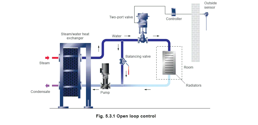
The system consists of a proportional controller with an outside sensor sensing ambient air temperature. The controller might be set with a fairly large proportional band, such that at an ambient temperature of -1°C the valve is full open, and at an ambient of 19°C the valve is fully closed. As the ambient temperature will have an effect on the heat loss from the building, it is hoped that the room temperature will be controlled.
However, there is no feedback regarding the room temperature and heating due to other factors.
In mild weather, although the flow of water is being controlled, other factors, such as high solar gain, might cause the room to overheat. In other words, open control tends only to provide a coarse control of the application.
Figure 5.3.2 depicts a slightly more sophisticated control system with two sensors.
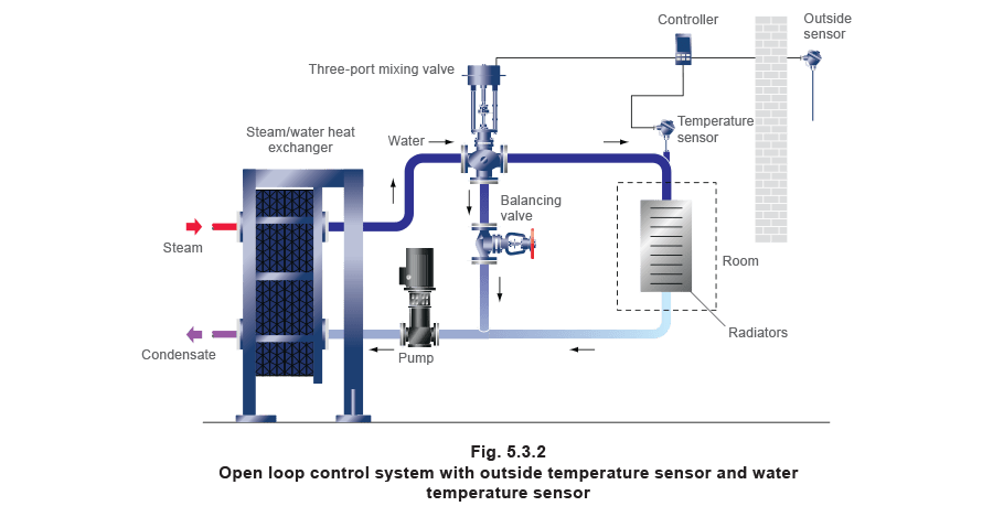
The system uses a three-port mixing valve with an actuator, controller and outside air sensor, plus a temperature sensor in the water line.
The outside temperature sensor provides a remote set point input to the controller, which is used to offset the water temperature set point. In this way, closed loop control applies to the water temperature flowing through the radiators.
When it is cold outside, water flows through the radiator at its maximum temperature. As the outside temperature rises, the controller automatically reduces the temperature of the water flowing through the radiators.
However, this is still open loop control as far as the room temperature is concerned, as there is no feedback from the building or space being heated. If radiators are oversized or design errors have occurred, overheating will still occur.
Closed loop control
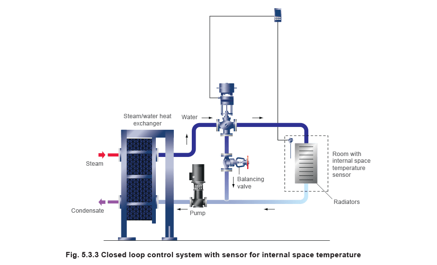
Quite simply, a closed loop control requires feedback; information sent back direct from the process or system. Using the simple heating system shown in Figure 5.3.3, the addition of an internal space temperature sensor will detect the room temperature and provide closed loop control with respect to the room.
In Figure 5.3.3, the valve and actuator are controlled via a space temperature sensor in the room, providing feedback from the actual room temperature.
Disturbances
Disturbances are factors, which enter the process or system to upset the value of the controlled medium. These disturbances can be caused by changes in load or by outside influences.
For example; if in a simple heating system, a room was suddenly filled with people, this would constitute a disturbance, since it would affect the temperature of the room and the amount of heat required to maintain the desired space temperature.
Feedback control
This is another type of closed loop control. Feedback control takes account of disturbances and feeds this information back to the controller, to allow corrective action to be taken. For example, if a large number of people enter a room, the space temperature will increase, which will then cause the control system to reduce the heat input to the room.
Feed-forward control
With feed-forward control, the effects of any disturbances are anticipated and allowed for before the event actually takes place.
An example of this is bringing the boiler up to high fire before bringing a large steam-using process plant on line. The sequence of events might be that the process plant is switched on. This action, rather than opening the steam valve to the process, instructs the boiler burner to high fire. Only when the high fire position is reached is the process steam valve allowed to open, and then in a slow, controlled way.
Single loop control
This is the simplest control loop involving just one controlled variable, for instance, temperature. To explain this, a steam-to-water heat exchanger is considered as shown in Figure 5.3.4.
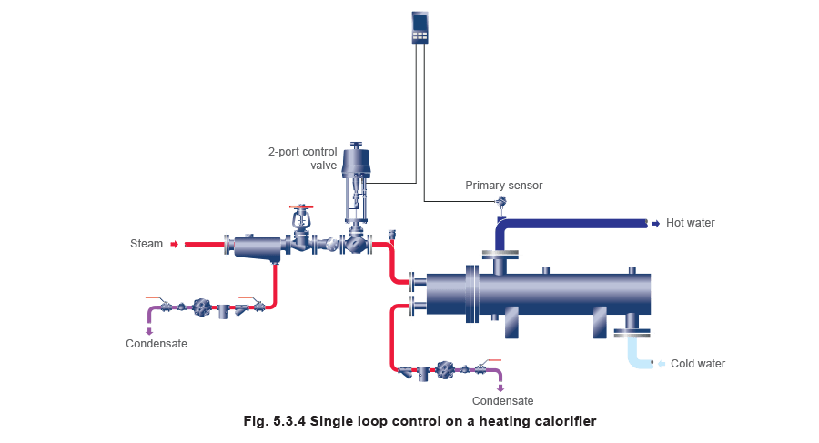
The only one variable controlled in Figure 5.3.4 is the temperature of the water leaving the heat exchanger. This is achieved by controlling the 2-port steam valve supplying steam to the heat exchanger. The primary sensor may be a thermocouple or PT100 platinum resistance thermometer sensing the water temperature.
The controller compares the signal from the sensor to the set point on the controller. If there is a difference, the controller sends a signal to the actuator of the valve, which in turn moves the valve to a new position. The controller may also include an output indicator, which shows the percentage of valve opening.
Single control loops provide the vast majority of control for heating systems and industrial processes.
Other terms used for single control loops include:
- Set value control
- Single closed loop control.
- Feedback control.
Multi-loop control
The following example considers an application for a slow moving timber-based product, which must be controlled to a specific humidity level (see Figures 5.3.5 and 5.3.6).
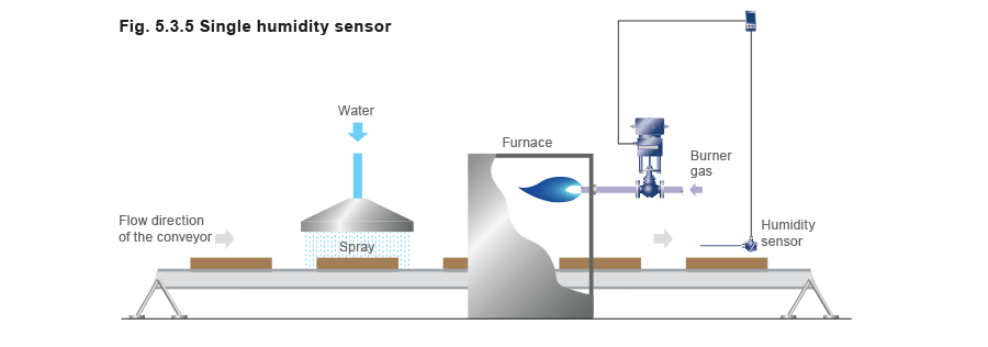
In Figure 5.3.5, the single humidity sensor at the end of the conveyor controls the amount of heat added by the furnace. But if the water spray rate changes due, for instance, to fluctuations in the water supply pressure, it may take perhaps 10 minutes before the product reaches the far end of the conveyor and the humidity sensor reacts. This will cause variations in product quality.
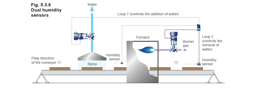
To improve the control, a second humidity sensor on another control loop can be installed immediately after the water spray, as shown in Figure 5.3.6. This humidity sensor provides a remote set point input to the controller which is used to offset the local set point. The local set point is set at the required humidity after the furnace. This, in a simple form, illustrates multi-loop control.
This humidity control system consists of two control loops:
- Loop 1 controls the addition of water.
- Loop 2 controls the removal of water.
Within this process, factors will influence both loops. Some factors such as water pressure will affect both loops. Loop 1 will try to correct for this, but any resulting error will have an impact on Loop 2
Cascade control
Where two independent variables need to be controlled with one valve, a cascade control system may be used.
Figure 5.3.7 shows a steam jacketed vessel full of liquid product. The essential aspects of the process are quite rigorous:
- The product in the vessel must be heated to a certain temperature.
- The steam must not exceed a certain temperature or the product may be spoiled
- The product temperature must not increase faster than a certain rate or the product may be spoiled.
If a normal, single loop control was used with the sensor in the liquid, at the start of the process the sensor would detect a low temperature, and the controller would signal the valve to move to the fully open position. This would result in a problem caused by an excessive steam temperature in the jacket.

The solution is to use a cascade control using two controllers and two sensors:
- A slave controller (Controller 2) and sensor monitoring the steam temperature in the jacket, and outputting a signal to the control valve
- A master controller (Controller 1) and sensor monitoring the product temperature with the controller output directed to the slave controller.
- The output signal from the master controller is used to vary the set point in the slave controller, ensuring that the steam temperature is not exceeded.
Example 5.3.1 An example of cascade control applied to a process vessel
The liquid temperature is to be heated from 15°C to 80°C and maintained at 80°C for two hours.
The steam temperature cannot exceed 120°C under any circumstances.
The product temperature must not increase faster than 1°C/minute.
The master controller can be ramped so that the rate of increase in water temperature is not higher than that specified.
The master controller is set in reverse acting mode, so that its output signal to the slave controller is 20 mA at low temperature and 4 mA at high temperature.
The remote set point on the slave controller is set so that its output signal to the valve is 4 mA when the steam temperature is 80°C, and 20 mA when the steam temperature is 120°C. In this way, the temperature of the steam cannot be higher than that tolerated by the system, and the steam pressure in the jacket cannot be higher than the, 1 bar g, saturation pressure at 120°C.
Dynamics of the process
This is a very complex subject but this part of the text will cover the most basic considerations.
The term ‘time constant’, which deals with the definition of the time taken for actuator movement, has already been outlined in Module 5.1; but to reiterate, it is the time taken for a control system to reach approximately two-thirds of its total movement as a result of a given step change in temperature, or other variable.
Other parts of the control system will have similar time based responses - the controller and its components and the sensor itself. All instruments have a time lag between the input to the instrument and its subsequent output. Even the transmission system will have a time lag - not a problem with electric/electronic systems but a factor that may need to be taken into account with pneumatic transmission systems.
Figures 5.3.8 and 5.3.9 show some typical response lags for a thermocouple that has been installed into a pocket for sensing water temperature.

Apart from the delays in sensor response, other parts of the control system also affect the response time. With pneumatic and self-acting systems, the valve/actuator movement tends to be smooth and, in a proportional controller, directly proportional to the temperature deviation at the sensor.
With an electric actuator there is a delay due to the time it takes for the motor to move the control linkage. Because the control signal is a series of pulses, the motor provides bursts of movement followed by periods where the actuator is stationary. The response diagram (Figure 5.3.10) depicts this. However, because of delays in the process response, the final controlled temperature can still be smooth.

The control systems covered in this Module have only considered steady state conditions. However the process or plant under control may be subject to variations following a certain behaviour pattern. The control system is required to make the process behave in a predictable manner. If the process is one which changes rapidly, then the control system must be able to react quickly.
If the process undergoes slow change, the demands on the operating speed of the control system are not so stringent.
Much is documented about the static and dynamic behaviour of controllers and control systems - sensitivity, response time and so on. Possibly the most important factor of consideration is the time lag of the complete control loop.
The dynamics of the process need consideration to select the right type of controller, sensor and actuator.
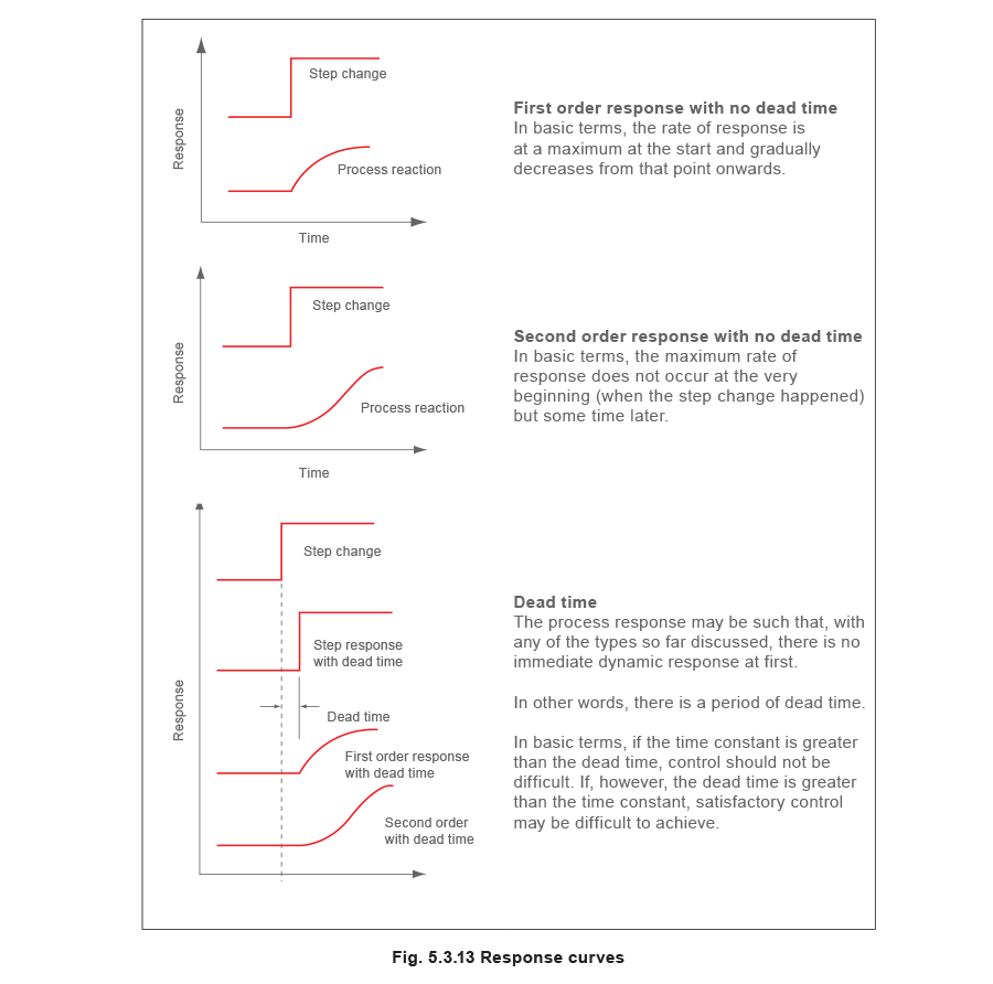
Process reactions
These dynamic characteristics are defined by the reaction of the process to a sudden change in the control settings, known as a step input. This might include an immediate change in set temperature, as shown in Figure 5.3.11.
The response of the system is depicted in Figure 5.3.12, which shows a certain amount of dead time before the process temperature starts to increase. This dead time is due to the control lag caused by such things as an electrical actuator moving to its new position. The time constant will differ according to the dynamic response of the system, affected by such things as whether or not the sensor is housed in a pocket.

The response of any two processes can have different characteristics because of the system.
The effects of dead time and the time constant on the system response to a sudden input change are shown graphically in Figure 5.3.12.
Systems that have a quick initial rate of response to input changes are generally referred to as possessing a first order response.
Systems that have a slow initial rate of response to input changes are generally referred to as possessing a second order response.
An overview of the basic types of process response (effects of dead time, first order response, and second order response) is shown in Figure 5.3.13.