Basic Control Theory

Contents
Basic Control Theory
This tutorial looks at on/off and continuous control modes.
It introduces proportional, integral and derivitive control actions and explains some of the terminology.
Modes of control
An automatic temperature control might consist of a valve, actuator, controller and sensor detecting the space temperature in a room. The control system is said to be ‘in balance’ when the space temperature sensor does not register more or less temperature than that required by the control system. What happens to the control valve when the space sensor registers a change in temperature (a temperature deviation) depends on the type of control system used. The relationship between the movement of the valve and the change of temperature in the controlled medium is known as the mode of control or control action.
There are two basic modes of control:
Variations of both these modes exist, which will now be examined in greater detail.
On/off control
Occasionally known as two-step or two-position control, this is the most basic control mode.
Considering the tank of water shown in Figure 5.2.1, the objective is to heat the water in the tank using the energy given off a simple steam coil. In the flow pipe to the coil, a two-port valve and actuator is fitted, complete with a thermostat, placed in the water in the tank.
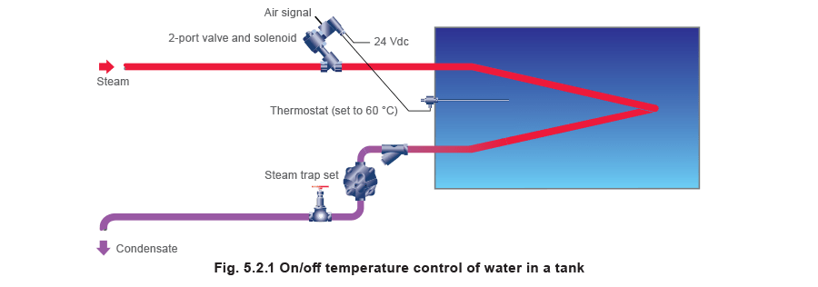
The thermostat is set to 60°C, which is the required temperature of the water in the tank. Logic dictates that if the switching point were actually at 60°C the system would never operate properly, because the valve would not know whether to be open or closed at 60°C. From then on it could open and shut rapidly, causing wear.
For this reason, the thermostat would have an upper and lower switching point. This is essential to prevent over-rapid cycling. In this case the upper switching point might be 61°C (the point at which the thermostat tells the valve to shut) and the lower switching point might be 59°C (the point when the valve is told to open). Thus there is an in-built switching difference in the thermostat of ±1°C about the 60°C set point.
This 2°C (±1°C) is known as the switching differential. (This will vary between thermostats). A diagram of the switching action of the thermostat would look like the graph shown in Figure 5.2.2.
The temperature of the tank contents will fall to 59°C before the valve is asked to open and will rise to 61°C before the valve is instructed to close.

Figure 5.2.2 shows straight switching lines but the effect on heat transfer from coil to water will not be immediate. It will take time for the steam in the coil to affect the temperature of the water in the tank. Not only that, but the water in the tank will rise above the 61°C upper limit and fall below the 59°C lower limit. This can be explained by cross referencing Figures 5.2.2 and 5.2.3. First however it is necessary to describe what is happening.
At point A (59°C, Figure 5.2.3) the thermostat switches on, directing the valve wide open. It takes time for the transfer of heat from the coil to affect the water temperature, as shown by the graph of the water temperature in Figure 5.2.3. At point B (61°C) the thermostat switches off and allows the valve to shut. However the coil is still full of steam, which continues to condense and give up its heat.
Hence the water temperature continues to rise above the upper switching temperature, and ‘overshoots’ at C, before eventually falling.
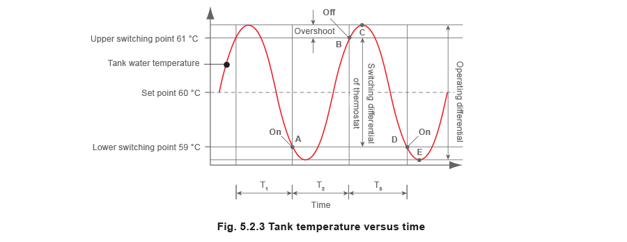
From this point onwards, the water temperature in the tank continues to fall until, at point D (59°C), the thermostat tells the valve to open. Steam is admitted through the coil but again, it takes time to have an effect and the water temperature continues to fall for a while, reaching its trough of undershoot at point E.
The difference between the peak and the trough is known as the operating differential. The switching differential of the thermostat depends on the type of thermostat used. The operating differential depends on the characteristics of the application such as the tank, its contents, the heat transfer characteristics of the coil, the rate at which heat is transferred to the thermostat, and so on.
Essentially, with on / off control, there are upper and lower switching limits, and the valve is either fully open or fully closed - there is no intermediate state.
However, controllers are available that provide a proportioning time control, in which it is possible to alter the ratio of the ‘on’ time to the ‘off’ time to control the controlled condition. This proportioning action occurs within a selected bandwidth around the set point; the set point being the bandwidth mid point.
If the controlled condition is outside the bandwidth, the output signal from the controller is either fully on or fully off, acting as an on / off device. If the controlled condition is within the bandwidth, the controller output is turned on and off relative to the deviation between the value of the controlled condition and the set point.
With the controlled condition being at set point, the ratio of ‘on’ time to ‘off’ time is 1:1, that is, the ‘on’ time equals the ‘off’ time. If the controlled condition is below the set point, the ‘on’ time will be longer than the ‘off’ time, whilst if above the set point, the ‘off’ time will be longer, relative to the deviation within the bandwidth.
The main advantages of on / off control are that it is simple and very low cost. This is why it is frequently found on domestic type applications such as central heating boilers and heater fans.
Its major disadvantage is that the operating differential might fall outside the control tolerance required by the process. For example, on a food production line, where the taste and repeatability of taste is determined by precise temperature control, on / off control could well be unsuitable.
By contrast, in the case of space heating there are often large storage capacities (a large area to heat or cool that will respond to temperature change slowly) and slight variation in the desired value is acceptable. In many cases on / off control is quite appropriate for this type of application.
If on/off control is unsuitable because more accurate temperature control is required, the next option is continuous control.
Continuous control
Continuous control is often called modulating control. It means that the valve is capable of moving continually to change the degree of valve opening or closing. It does not just move to either fully open or fully closed, as with on / off control.
There are three basic control actions that are often applied to continuous control:
It is also necessary to consider these in combination such as P + I, P + D, P + I + D. Although it is possible to combine the different actions, and all help to produce the required response, it is important to remember that both the integral and derivative actions are usually corrective functions of a basic proportional control action.
The three control actions are considered below.
Proportional control
This is the most basic of the continuous control modes and is usually referred to by use of the letter ‘P’. The principle aim of proportional control is to control the process as the conditions change.
This section shows that:
- The larger the proportional band, the more stable the control, but the greater the offset.
- The narrower the proportional band, the less stable the process, but the smaller the offset.
- The aim, therefore, should be to introduce the smallest acceptable proportional band that will always keep the process stable with the minimum offset.
In explaining proportional control, several new terms must be introduced.
To define these, a simple analogy can be considered - a cold water tank is supplied with water via a float operated control valve and with a globe valve on the outlet pipe valve ‘V’, as shown in Figure 5.2.4. Both valves are the same size and have the same flow capacity and flow characteristic.
The desired water level in the tank is at point B (equivalent to the set point of a level controller).
It can be assumed that, with valve ‘V’ half open, (50% load) there is just the right flowrate of water entering via the float operated valve to provide the desired flow out through the discharge pipe, and to maintain the water level in the tank at point at B.
The system can be said to be in balance (the flowrate of water entering and leaving the tank is the same); under control, in a stable condition (the level is not varying) and at precisely the desired water level (B); giving the required outflow.
With the valve ‘V’ closed, the level of water in the tank rises to point A and the float operated valve cuts off the water supply (see Figure 5.2.5 below).
The system is still under control and stable but control is above level B. The difference between level B and the actual controlled level, A, is related to the proportional band of the control system.
Once again, if valve ‘V’ is half opened to give 50% load, the water level in the tank will return to the desired level, point B.

Figure 5.2.6 below, the valve ‘V’ is fully opened (100% load). The float operated valve will need to drop to open the inlet valve wide and admit a higher flowrate of water to meet the increased demand from the discharge pipe. When it reaches level C, enough water will be entering to meet the discharge needs and the water level will be maintained at point C.

The system is under control and stable, but there is an offset; the deviation in level between points B and C. Figure 5.2.7 combines the three conditions used in this example.
The difference in levels between points A and C is known as the Proportional Band or P-band, since this is the change in level (or temperature in the case of a temperature control) for the control valve to move from fully open to fully closed.
One recognised symbol for Proportional Band is Xp.
The analogy illustrates several basic and important points relating to proportional control:
- The control valve is moved in proportion to the error in the water level (or the temperature deviation, in the case of a temperature control) from the set point
- The set point can only be maintained for one specific load condition.
- Whilst stable control will be achieved between points A and C, any load causing a difference in level to that of B will always provide an offset.

Note: By altering the fulcrum position, the system Proportional Band changes. Nearer the float gives a narrower P-band, whilst nearer the valve gives a wider P-band.
Figure 5.2.8 illustrates why this is so. Different fulcrum positions require different changes in water level to move the valve from fully open to fully closed. In both cases, It can be seen that level B represents the 50% load level, A represents the 0% load level, and C represents the 100% load level. It can also be seen how the offset is greater at any same load with the wider proportional band.

The examples depicted in Figures 5.2.4 through to 5.2.8 describe proportional band as the level (or perhaps temperature or pressure etc.) change required to move the valve from fully open to fully closed. This is convenient for mechanical systems, but a more general (and more correct) definition of proportional band is the percentage change in measured value required to give a 100% change in output. It is therefore usually expressed in percentage terms rather than in engineering units such as degrees centigrade.
For electrical and pneumatic controllers, the set value is at the middle of the proportional band.
The effect of changing the P-band for an electrical or pneumatic system can be described with a slightly different example, by using a temperature control.
The space temperature of a building is controlled by a water (radiator type) heating system using a proportional action control by a valve driven with an electrical actuator, and an electronic controller and room temperature sensor. The control selected has a proportional band (P-band or Xp) of 6% of the controller input span of 0° - 100°C, and the desired internal space temperature is 18°C.
Under certain load conditions, the valve is 50% open and the required internal temperature is correct at 18°C.
A fall in outside temperature occurs, resulting in an increase in the rate of heat loss from the building. Consequently, the internal temperature will decrease. This will be detected by the room temperature sensor, which will signal the valve to move to a more open position allowing hotter water to pass through the room radiators.
The valve is instructed to open by an amount proportional to the drop in room temperature. In simplistic terms, if the room temperature falls by 1°C, the valve may open by 10%; if the room temperature falls by 2°C, the valve will open by 20%.
In due course, the outside temperature stabilises and the inside temperature stops falling. In order to provide the additional heat required for the lower outside temperature, the valve will stabilise in a more open position; but the actual inside temperature will be slightly lower than 18°C.
Example 5.2.1 and Figure 5.2.9 explain this further, using a P-band of 6°C.
Example 5.2.1 Consider a space heating application with the following characteristics:
- The required temperature in the building is 18°C.
- The room temperature is currently 18°C, and the valve is 50% open.
- The proportional band is set at 6% of 100°C = 6°C, which gives 3°C either side of the 18°C set point.
Figure 5.2.9 shows the room temperature and valve relationship:
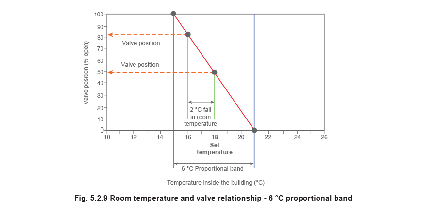
As an example, consider the room temperature falling to 16 °C. This is a 2 °C drop of a 6 °C proportional band, in other words, 33.3% of proportional band. Therefore the control valve must open by a further 33% to 83%, as shown in Figure 5.2.9.
With proportional control, if the load changes, so too will the offset:
- A load of less than 50% will cause the room temperature to be above the set value.
- A load of more than 50% will cause the room temperature to be below the set value.
The deviation between the set temperature on the controller (the set point) and the actual room temperature is called the ‘proportional offset’.
In Example 5.2.1, as long as the load conditions remain the same, the control will remain steady at a valve opening of 83.3%; this is called ‘sustained offset’.
The effect of adjusting the P-band
In electronic and pneumatic controllers, the P-band is adjustable. This enables the user to find a setting suitable for the individual application.
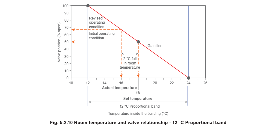
Increasing the P-band - For example, if the previous application had been programmed with a 12% proportional band equivalent to 12°C, the results can be seen in Figure 5.2.10. Note that the wider P-band results in a less steep ‘gain’ line. For the same change in room temperature the valve movement will be smaller. The term ‘gain’ is discussed in a following section.
In this instance, the 2°C fall in room temperature would give a valve opening of about 68% from the chart in Figure 5.2.10.
Reducing the P-band - Conversely, if the P-band is reduced, the valve movement per temperature increment is increased. However, reducing the P-band to zero gives an on / off control. The ideal P-band is as narrow as possible without producing a noticeable oscillation in the actual room temperature.
Gain
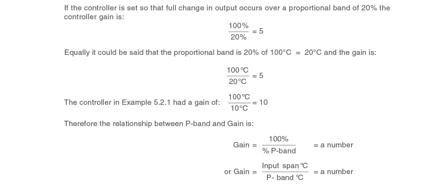
The term ‘gain’ is often used with controllers and is simply the reciprocal of proportional band.
The larger the controller gain, the more the controller output will change for a given error. For instance for a gain of 1, an error of 10% of scale will change the controller output by 10% of scale, for a gain of 5, an error of 10% will change the controller output by 50% of scale, whilst for a gain of 10, an error of 10% will change the output by 100% of scale.
The proportional band in ‘degree terms’ will depend on the controller input scale. For instance, for a controller with a 200°C input scale:
An Xp of 20% = 20% of 200°C = 40°C
An Xp of 10% = 10% of 200°C = 20°C The Steam and Condensate Loop 5.2.8
Example 5.2.2
Let the input span of a controller be 100°C.
As a reminder:
- A wide proportional band (small gain) will provide a less sensitive response, but a greater stability.
- A narrow proportional band (large gain) will provide a more sensitive response, but there is a practical limit to how narrow the Xp can be set.
- Too narrow a proportional band (too much gain) will result in oscillation and unstable control.
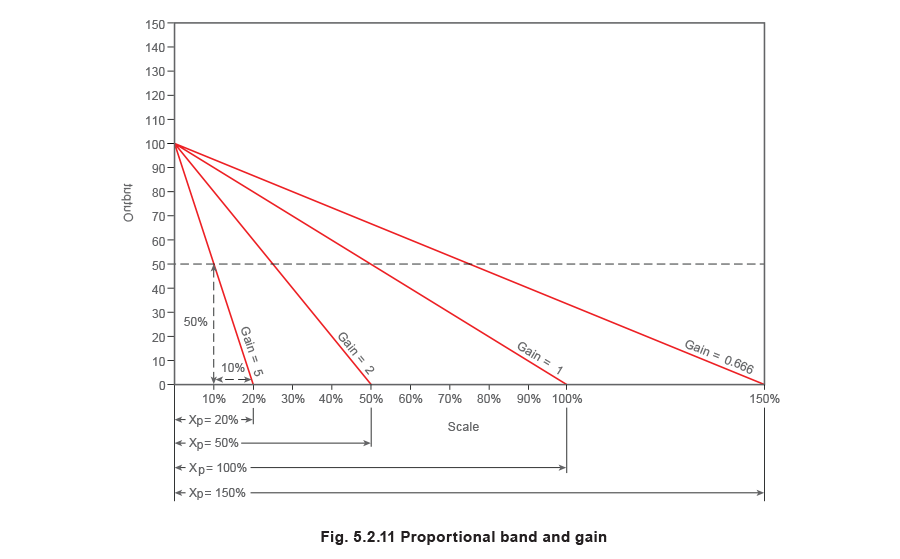
For any controller for various P-bands, gain lines can be determined as shown in Figure 5.2.11, where the controller input span is 100°C.
Reverse or direct acting control signal
A closer look at the figures used so far to describe the effect of proportional control shows that the output is assumed to be reverse acting. In other words, a rise in process temperature causes the control signal to fall and the valve to close. This is usually the situation on heating controls. This configuration would not work on a cooling control; here the valve must open with a rise in temperature. This is termed a direct acting control signal. Figures 5.2.12 and 5.2.13 depict the difference between reverse and direct acting control signals for the same valve action.

On mechanical controllers (such as a pneumatic controller) it is usual to be able to invert the output signal of the controller by rotating the proportional control dial. Thus, the magnitude of the proportional band and the direction of the control action can be determined from the same dial.
On electronic controllers, reverse acting (RA) or direct acting (DA) is selected through the keypad.
Gain line offset or proportional effect
From the explanation of proportional control, it should be clear that there is a control offset or a deviation of the actual value from the set value whenever the load varies from 50%.
To further illustrate this, consider Example 5.2.1 with a 12°C P-band, where an offset of 2°C was expected. If the offset cannot be tolerated by the application, then it must be eliminated.
This could be achieved by relocating (or resetting) the set point to a higher value. This provides the same valve opening after manual reset but at a room temperature of 18°C not 16°C.

Manual reset
The offset can be removed either manually or automatically. The effect of manual reset can be seen in Figure 5.2.14, and the value is adjusted manually by applying an offset to the set point of 2°C.
It should be clear from Figure 5.2.14 and the above text that the effect is the same as increasing the set value by 2°C. The same valve opening of 66.7% now coincides with the room temperature at 18°C.
The effects of manual reset are demonstrated in Figure 5.2.15.

Integral control - automatic reset action
Manual reset’ is usually unsatisfactory in process plant where each load change will require a reset action. It is also quite common for an operator to be confused by the differences between:
- Set value - What is on the dial.
- Actual value - What the process value is.
- Required value - The perfect process condition.
Such problems are overcome by the reset action being contained within the mechanism of an automatic controller.
Such a controller is primarily a proportional controller. It then has a reset function added, which is called ‘integral action’. Automatic reset uses an electronic or pneumatic integration routine to perform the reset function. The most commonly used term for automatic reset is integral action, which is given the letter I.
The function of integral action is to eliminate offset by continuously and automatically modifying the controller output in accordance with the control deviation integrated over time. The Integral Action Time (IAT) is defined as the time taken for the controller output to change due to the integral action to equal the output change due to the proportional action. Integral action gives a steadily increasing corrective action as long as an error continues to exist. Such corrective action will increase with time and must therefore, at some time, be sufficient to eliminate the steady state error altogether, providing sufficient time elapses before another change occurs. The controller allows the integral time to be adjusted to suit the plant dynamic behaviour.
Proportional plus integral (P + I) becomes the terminology for a controller incorporating these features.
The integral action on a controller is often restricted to within the proportional band.
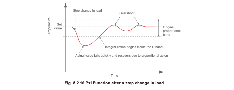
A typical P + I response is shown in Figure 5.2.16, for a step change in load.
The IAT is adjustable within the controller:
- If it is too short, over-reaction and instability will result.
- If it is too long, reset action will be very slow to take effect.
IAT is represented in time units. On some controllers the adjustable parameter for the integral action is termed ‘repeats per minute’, which is the number of times per minute that the integral action output changes by the proportional output change.
- Repeats per minute =1/(IAT in minutes)
- IAT = Infinity – Means no integral action
- IAT = 0 – Means infinite integral action
It is important to check the controller manual to see how integral action is designated.
Overshoot and ‘wind up’
With P + I controllers (and with P controllers), overshoot is likely to occur when there are time lags on the system.
A typical example of this is after a sudden change in load. Consider a process application where a process heat exchanger is designed to maintain water at a fixed temperature.
The set point is 80°C, the P-band is set at 5°C (±2.5°C), and the load suddenly changes such that the returning water temperature falls almost instantaneously to 60°C.
Figure 5.2.16 shows the effect of this sudden (step change) in load on the actual water temperature. The measured value changes almost instantaneously from a steady 80°C to a value of 60°C.
By the nature of the integration process, the generation of integral control action must lag behind the proportional control action, introducing a delay and more dead time to the response. This could have serious consequences in practice, because it means that the initial control response, which in a proportional system would be instantaneous and fast acting, is now subjected to a delay and responds slowly. This may cause the actual value to run out of control and the system to oscillate. These oscillations may increase or decrease depending on the relative values of the controller gain and the integral action. If applying integral action it is important to make sure, that it is necessary and if so, that the correct amount of integral action is applied.
Integral control can also aggravate other situations. If the error is large for a long period, for example after a large step change or the system being shut down, the value of the integral can become excessively large and cause overshoot or undershoot that takes a long time to recover. To avoid this problem, which is often called ‘integral wind-up’, sophisticated controllers will inhibit integral action until the system gets fairly close to equilibrium.
To remedy these situations it is useful to measure the rate at which the actual temperature is changing; in other words, to measure the rate of change of the signal. Another type of control mode is used to measure how fast the measured value changes, and this is termed Rate Action or Derivative Action.
Derivative control - rate action
A Derivative action (referred to by the letter D) measures and responds to the rate of change of process signal, and adjusts the output of the controller to minimise overshoot.
If applied properly on systems with time lags, derivative action will minimise the deviation from the set point when there is a change in the process condition. It is interesting to note that derivative action will only apply itself when there is a change in process signal. If the value is steady, whatever the offset, then derivative action does not occur.
One useful function of the derivative function is that overshoot can be minimised especially on fast changes in load. However, derivative action is not easy to apply properly; if not enough is used, little benefit is achieved, and applying too much can cause more problems than it solves.
D action is again adjustable within the controller, and referred to as TD in time units:
TD = 0 – Means no D action.
TD = Infinity – Means infinite D action.
P + D controllers can be obtained, but proportional offset will probably be experienced. It is worth remembering that the main disadvantage with a P control is the presence of offset. To overcome and remove offset, ‘I’ action is introduced. The frequent existence of time lags in the control loop explains the need for the third action D. The result is a P + I + D controller which, if properly tuned, can in most processes give a rapid and stable response, with no offset and without overshoot.
PID controllers
P and I and D are referred to as ‘terms’ and thus a P + I + D controller is often referred to as a three term controller.
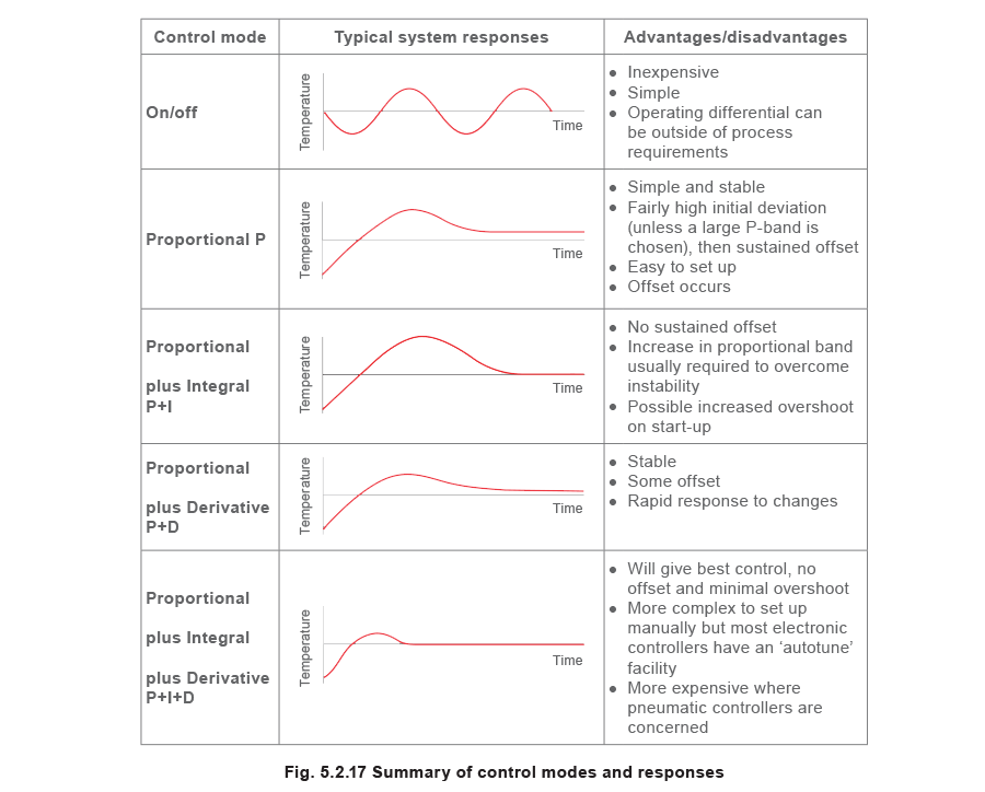
Summary of modes of control
The various characteristics can be summarised, as shown in Figure 5.2.17.
Finally, the controls engineer must try to avoid the danger of using unnecessarily complicated controls for a specific application. The least complicated control action, which will provide the degree of control required, should always be selected.
Further terminology
Time constant
This is defined as: ‘The time taken for a controller output to change by 63.2% of its total due to a step (or sudden) change in process load’.
In reality, the explanation is more involved because the time constant is really the time taken for a signal or output to achieve its final value from its initial value, had the original rate of increase been maintained. This concept is depicted in Figure 5.12.18.

Example 5.2.2 A practical appreciation of the time constant
Consider two tanks of water, tank A at a temperature of 25°C, and tank B at 75°C. A sensor is placed in tank A and allowed to reach equilibrium temperature. It is then quickly transferred to tank B. The temperature difference between the two tanks is 50°C, and 63.2% of this temperature span can be calculated as shown below:
63.2% of 50°C = 31.6°C
The initial datum temperature was 25°C, consequently the time constant for this simple example is the time required for the sensor to reach 56.6°C, as shown below:
25°C + 31.6°C = 56.6°C
Hunting
Often referred to as instability, cycling or oscillation. Hunting produces a continuously changing deviation from the normal operating point. This can be caused by:
- The proportional band being too narrow.
- The integral time being too short.
- The derivative time being too long.
- A combination of these.
Long time constants or dead times in the control system or the process itself
In Figure 5.2.19 the heat exchanger is oversized for the application. Accurate temperature control will be difficult to achieve and may result in a large proportional band in an attempt to achieve stability.
If the system load suddenly increases, the two-port valve will open wider, filling the heat exchanger with high temperature steam. The heat transfer rate increases extremely quickly causing the water system temperature to overshoot. The rapid increase in water temperature is picked up by the sensor and directs the two-port valve to close quickly. This causes the water temperature to fall, and the two-port valve to open again. This cycle is repeated, the cycling only ceasing when the PID terms are adjusted. The following example (Example 5.2.3) gives an idea of the effects of a hunting steam system.

Example 5.2.3 The effect of hunting on the system in Figure 5.2.19
Consider the steam to water heat exchanger system in Figure 5.2.19. Under minimum load conditions, the size of the heat exchanger is such that it heats the constant flowrate secondary water from 60°C to 65°C with a steam temperature of 70°C. The controller has a set point of 65°C and a P-band of 10°C.
Consider a sudden increase in the secondary load, such that the returning water temperature almost immediately drops by 40°C. The temperature of the water flowing out of the heat exchanger will also drop by 40°C to 25°C. The sensor detects this and, as this temperature is below the P-band, it directs the pneumatically actuated steam valve to open fully.
The steam temperature is observed to increase from 70°C to 140°C almost instantaneously. What is the effect on the secondary water temperature and the stability of the control system?
As demonstrated in Module 13.2 (The heat load, heat exchanger and steam load relationship), the heat exchanger temperature design constant, TDC, can be calculated from the observed operating conditions and Equation 13.2.2:

In this example, the observed conditions (at minimum load) are as follows:

When the steam temperature rises to 140°C, it is possible to predict the outlet temperature from Equation 13.2.5:

The heat exchanger outlet temperature is 80°C, which is now above the P-band, and the sensor now signals the controller to shut down the steam valve.
The steam temperature falls rapidly, causing the outlet water temperature to fall; and the steam valve opens yet again. The system cycles around these temperatures until the control parameters are changed. These symptoms are referred to as ‘hunting’. The control valve and its controller are hunting to find a stable condition. In practice, other factors will add to the uncertainty of the situation, such as the system size and reaction to temperature change and the position of the sensor.
Hunting of this type can cause premature wear of system components, in particular valves and actuators, and gives poor control.
Example 5.2.3 is not typical of a practical application. In reality, correct design and sizing of the control system and steam heated heat exchanger would not be a problem.
Lag
Lag is a delay in response and will exist in both the control system and in the process or system under control.
Consider a small room warmed by a heater, which is controlled by a room space thermostat. A large window is opened admitting large amounts of cold air. The room temperature will fall but there will be a delay while the mass of the sensor cools down to the new temperature - this is known as control lag. The delay time is also referred to as dead time.
Having then asked for more heat from the room heater, it will be some time before this takes effect and warms up the room to the point where the thermostat is satisfied. This is known as system lag or thermal lag.
Rangeability
This relates to the control valve and is the ratio between the maximum controllable flow and the minimum controllable flow, between which the characteristics of the valve (linear, equal percentage, quick opening) will be maintained. With most control valves, at some point before the fully closed position is reached, there is no longer a defined control over flow in accordance with the valve characteristics. Reputable manufacturers will provide rangeability figures for their valves.
Turndown ratio
Turndown ratio is the ratio between the maximum flow and the minimum controllable flow. It will be substantially less than the valve’s rangeability if the valve is oversized.
Although the definition relates only to the valve, it is a function of the complete control system.