Steam Engineering Principles and Heat Transfer

Contents
Entropy - A Basic Understanding
Entropy is a concept some find difficult to grasp, but in truth it does not deserve such notoriety. Look upon Entropy as a road map that connects thermodynamic situations. This tutorial hopes to shed some light on this subject, by approaching it from first principles.
What is entropy?
In some ways, it is easier to say what it is not! It is not a physical property of steam like pressure or temperature or mass. A sensor cannot detect it, and it does not show on a gauge. Rather, it must be calculated from things that can be measured. Entropy values can then be listed and used in calculations; in particular, calculations to do with steam flow, and the production of power using turbines or reciprocating engines.
It is, in some ways, a measure of the lack of quality or availability of energy, and of how energy tends always to spread out from a high temperature source to a wider area at a lower temperature level. This compulsion to spread out has led some observers to label entropy as ‘time’s arrow’. If the entropy of a system is calculated at two different conditions, then the condition at which the entropy is greater occurs at a later time. The increase of entropy in the overall system always takes place in the same direction as time flows.
That may be of some philosophical interest, but does not help very much in the calculation of actual values. A more practical approach is to define entropy as energy added to or removed from a system, divided by the mean absolute temperature over which the change takes place.
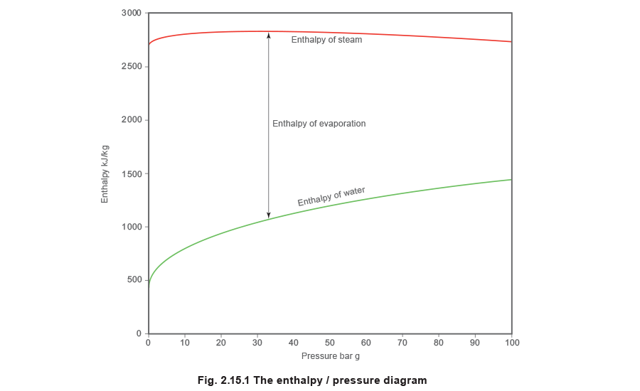
To see how this works, perhaps it is best to start off with a diagram showing how the enthalpy content of a kilogram of water increases as it is heated to different pressures and evaporated into steam.
Since the temperature and pressure at which water boils are in a fixed relationship to each other, Figure 2.15.1 could equally be drawn to show enthalpy against temperature, and then turned so that temperature became the vertical ordinates against a base of enthalpy, as in Figure 2.15.2.
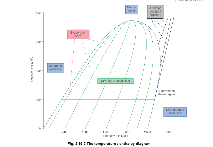
Lines of constant pressure originate on the saturated water line. The horizontal distance between the saturated water line and the dry saturated steam line represents the amount of latent heat or enthalpy of evaporation, and is called the evaporation line; (enthalpy of evaporation decreases with rising pressure). The area to the right of the dry saturated steam line is the superheated steam region, and lines of constant pressure now curve upwards as soon as they cross the dry saturated steam line.
A variation of the diagram in Figure 2.15.2, that can be extremely useful, is one in which the horizontal axis is not enthalpy but instead is enthalpy divided by the mean temperature at which the enthalpy is added or removed. To produce such a diagram, the entropy values can be calculated. By starting at the origin of the graph at a temperature of 0 °C at atmospheric pressure, and by adding enthalpy in small amounts, the graph can be built. As entropy is measured in terms of absolute temperature, the origin temperature of 0 °C is taken as 273.15 K. The specific heat of saturated water at this temperature is 4.228 kJ/kg K. For the purpose of constructing the diagram in Figure 2.15.3 the base temperature is taken as 273 K not 273.15 K.
By assuming a kilogram of water at atmospheric pressure, and by adding 4.228 kJ of energy, the water temperature would rise by 1 K from 273 K to 274 K. The mean temperature during this operation is 273.5 K, see Figure 2.15.3.
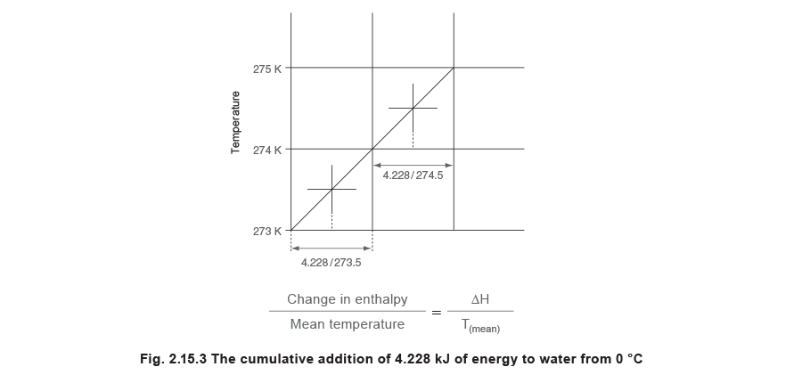
This value represents the change in enthalpy per degree of temperature rise for one kilogram of water and is termed the change in specific entropy. The metric units for specific entropy are therefore kJ/kg K.
This process can be continued by adding another 4.228 kJ of energy to produce a series of these points on a state point line. In the next increment, the temperature would rise from 274 K to 275 K, and the mean temperature is 274.5 K.

It can be seen from these simple calculations that, as the temperature increases, the change in entropy for each equal increment of enthalpy reduces slightly. If this incremental process were continuously repeated by adding more heat, it would be noticed that the change in entropy would continue to decrease. This is due to each additional increment of heat raising the temperature and so reducing the width of the elemental strip representing it. As more heat is added, so the state point line, in this case the saturated water line, curves gently upwards.
At 373.14 K (99.99 °C), the boiling point of water is reached at atmospheric pressure, and further additions of heat begin to boil off some of the water at this constant temperature. At this position, the state point starts to move horizontally across the diagram to the right, and is represented on Figure 2.15.4 by the horizontal evaporation line stretching from the saturated water line to the dry saturated steam line. Because this is an evaporation process, this added heat is referred to as enthalpy of evaporation.
At atmospheric pressure, steam tables state that the amount of heat added to evaporate 1 kg of water into steam is 2256.71 kJ. As this takes place at a constant temperature of 373.14 K, the mean temperature of the evaporation line is also 373.14 K.
The change in specific entropy from the water saturation line to the steam saturation line is therefore:

The diagram produced showing temperature against entropy would look something like that in Figure 2.15.4, where:
- 1 is the saturated water line.
- 2 is the dry saturated steam line.
- 3 are constant dryness fraction lines in the wet steam region.
- 4 are constant pressure lines in the superheat region.

What use is the temperature - entropy diagram (or T - S diagram)?
One potential use of the T - S diagram is to follow changes in the steam condition during processes occurring with no change in entropy between the initial and final state of the process. Such processes are termed Isentropic (constant entropy).
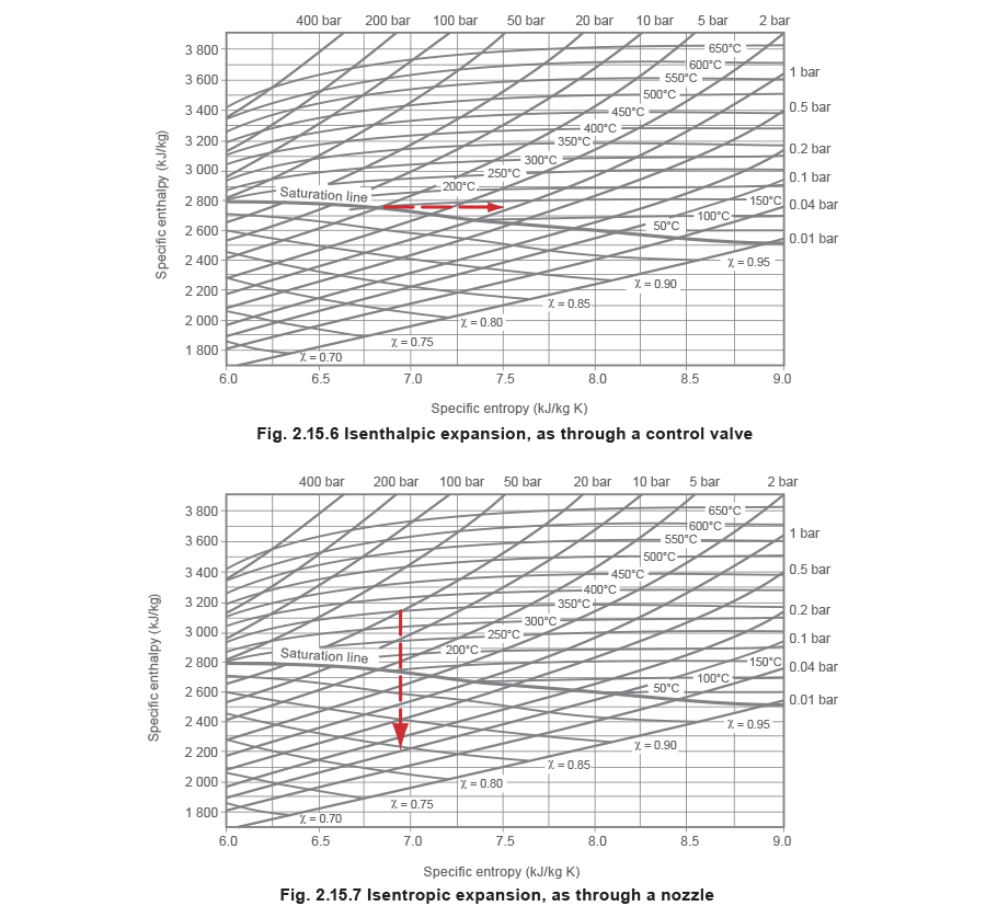
Unfortunately, the constant total heat lines shown in a T - S diagram are curved, which makes it difficult to follow changes in such free and unrestricted expansions as those when steam is allowed to flow through and expand after a control valve. In the case of a control valve, where the velocities in the connecting upstream and downstream pipes are near enough the same, the overall process occurs with constant enthalpy (isenthalpic). In the case of a nozzle, where the final velocity remains high, the overall process occurs with constant entropy.
To follow these different types of processes, a new diagram can be drawn complete with pressures and temperatures, showing entropy on the horizontal axis, and enthalpy on the vertical axis, and is called an enthalpy - entropy diagram, or H - S diagram, Figure 2.15.5.

The H - S diagram is also called the Mollier diagram or Mollier chart, named after Dr. Richard Mollier of Dresden who first devised the idea of such a diagram in 1904.
Now, the isenthalpic expansion of steam through a control valve is simply represented by a straight horizontal line from the initial state to the final lower pressure to the right of the graph, see Figure 2.15.6; and the isentropic expansion of steam through a nozzle is simply a line from the initial state falling vertically to the lower final pressure, see Figure 2.15.7.
An isentropic expansion of steam is always accompanied by a decrease in enthalpy, and this is referred to as the ‘heat drop’ (H) between the initial and final condition. The H values can be simply read at the initial and final points on the Mollier chart, and the difference gives the heat drop. The accuracy of the chart is sufficient for most practical purposes.
As a point of interest, as the expansion through a control valve orifice is an isenthalpic process, it is assumed that the state point moves directly to the right; as depicted in Figure 2.15.6. In fact, it does not do so directly. For the steam to squeeze through the narrow restriction it has to accelerate to a higher speed. It does so by borrowing energy from its enthalpy and converting it to kinetic energy. This incurs a heat drop. This part of the process is isentropic; the state point
moves vertically down to the lower pressure.
Having passed through the narrow restriction, the steam expands into the lower pressure region in the valve outlet, and eventually decelerates as the volume of the valve body increases to connect to the downstream pipe. This fall in velocity requires a reduction in kinetic energy which is mostly re-converted back into heat and re-absorbed by the steam. The heat drop that caused the initial increase in kinetic energy is reclaimed (except for a small portion lost due to the effects of friction), and on the H - S chart, the state point moves up the constant pressure line until it arrives at the same enthalpy value as the initial condition.
The path of the state point is to be seen in Figure 2.15.8, where pressure is reduced from 5 bar at saturation temperature to 1 bar via, for example, a pressure reducing valve. Steam’s enthalpy at the upstream condition of 5 bar is 2748 kJ/kg.
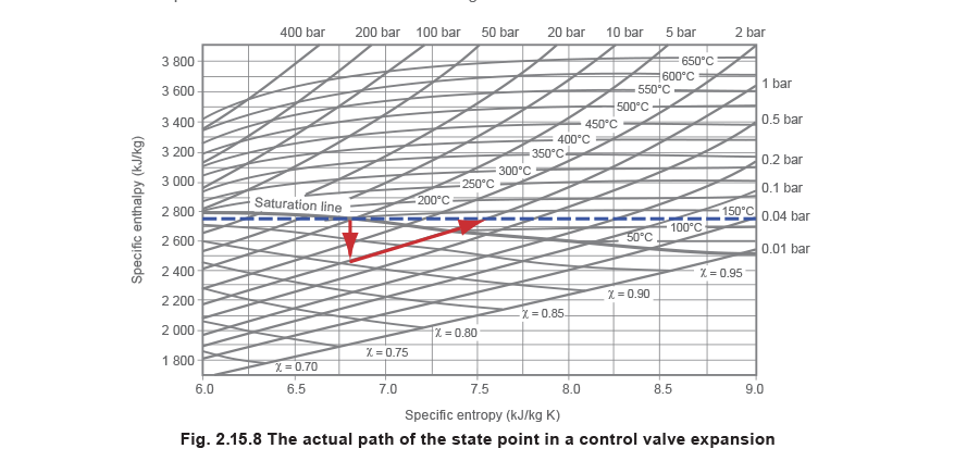
It is interesting to note that, in the example dicussed above and shown in Figure 2.15.8, the final condition of the steam is above the saturation line and is therefore superheated. Whenever such a process (commonly called a throttling process) takes place, the final condition of the steam will, in most cases, be drier than its initial condition. This will either produce drier saturated steam or superheated steam, depending on the respective positions of the initial and final state points.
The horizontal distance between the initial and final state points represents the change in entropy. In this example, although there was no overall change in enthalpy (ignoring the small effects of friction), the entropy increased from about 6.8 kJ/kg K to about 7.6 kJ/kg K.
Entropy always increases in a closed system
In any closed system, the overall change in entropy is always positive, that is, it will always increase. It is worth considering this in more detail, as it is fundamental to the concept of entropy. Whereas energy is always conserved (the first law of thermodynamics states that energy cannot be created or destroyed), the same cannot be said about entropy. The second law of thermodynamics says that whenever energy is exchanged or converted from one form
to another, the potential for energy to do work gets less. This really is what entropy is all about.
It is a measure of the lack of potential or quality of energy; and once that energy has been exchanged or converted, it cannot revert back to a higher state. The ultimate truth of this is that it is nature’s duty for all processes in the Universe to end up at the same temperature, so the entropy of the Universe is always increasing.
Example 2.15.1
Consider a teapot on a kitchen table that has just been filled with a certain quantity of water containing 200 kJ of heat energy at 100 °C (373 K) from an electric kettle. Consider next that the temperature of the air surrounding the mug is at 20 °C, and that the amount of heat in the teapot water would be 40 kJ at the end of the process. The second law of thermodynamics also states that heat will always flow from a hot body to a colder body, and in this example, it is certain that, if left for sufficient time, the teapot will cool to the same temperature as the air that surrounds it.
What are the changes in the entropy values for the overall process?

Practical applications - Heat exchangers
In a heat exchanger using saturated steam in the primary side to heat water from 20 °C to 60 °C in the secondary side, the steam will condense as it gives up its heat. This is depicted on the Mollier chart by the state point moving to the left of its initial position. For steady state conditions, dry saturated steam condenses at constant pressure, and the steam state point moves down the constant pressure line as shown in Figure 2.15.9.
Example 2.15.2
This example considers steam condensing from saturation at 2 bar at 120 °C with an entropy of 7.13 kJ/kg K, and an enthalpy of about 2700 kJ/kg. It can be seen that the state point moves from right to left, not horizontally, but by following the constant 2 bar pressure line. The chart is not big enough to show the whole condensing process but, if it were, it would show that the steam’s final state point would rest with an entropy of 1.53 kJ/kg K and an enthalpy of 504.8 kJ/kg, at 2 bar and 120 °C on the saturated water line.

It can be seen from Figure 2.15.9 that, when steam condenses, the state point moves down the evaporation line and the entropy is lowered. However, in any overall system, the entropy must increase, otherwise the second law of thermodynamics is violated; so how can this decrease in entropy be explained?
As for the teapot in the Example 2.15.1, this decrease in entropy only reflects what is happening in one part of the system. It must be remembered that any total system includes its surroundings, in Example 2.15.2, the water, which receives the heat imparted by the steam.
In Example 2.15.2, the water receives exactly the same amount of heat as the steam imparts (it is assumed there are no heat losses), but does so at a lower temperature than the steam; so, as entropy is given by enthalpy/temperature, dividing the same quantity of heat by a lower temperature means a greater gain in entropy by the water than is lost by the steam. There is therefore an overall gain in the system entropy, and an overall spreading out of energy.
Table 2.15.1 Relative densities/specific heat capacities of various solids
| Material | Relative density | Specific heat capacity kJ/kg °C |
| Aluminium | 2.55 - 2.80 | 0.92 |
| Andalusite | 0.71 | |
| Antimony | 0.2 | |
| Apatite | 0.83 | |
| Asbestos | 2.10 - 2.80 | 0.83 |
| Augite | 0.79 | |
| Bakelite, wood filler | 1.38 | |
| Bakelite, asbestos filler | 1.59 | |
| Barite | 4.5 | 0.46 |
| Barium | 3.5 | 2.93 |
| Basalt rock | 2.70 - 3.20 | 0.83 |
| Beryl | 0.83 | |
| Bismuth | 9.8 | 0.12 |
| Borax | 1.70 - 1.80 | 1 |
| Boron | 2.32 | 1.29 |
| Cadmium | 8.65 | 0.25 |
| Calcite, 0 - 37 °C | 0.79 | |
| Calcite, 0 - 100 °C | 0.83 | |
| Calcium | 4.58 | 0.62 |
| Carbon | 1.80 - 2.100 | 0.71 |
| Carborundum | 0.66 | |
| Cassiterite | 0.37 | |
| Cement, dry | 1.54 | |
| Cement, powder | 0.83 | |
| Charcoal | 1 | |
| Chalcopyrite | 0.54 | |
| Chromium | 7.1 | 0.5 |
| Clay | 1.80 - 2.60 | 0.92 |
| Coal | 0.64 - 0.93 | 1.08 - 1.54 |
| Cobalt | 8.9 | 0.46 |
| Concrete, stone | 0.79 | |
| Concrete, cinder | 0.75 | |
| Copper | 8.80 - 8.95 | 0.37 |
| Corundum | 0.41 | |
| Diamond | 3.51 | 0.62 |
| Dolomite rock | 2.9 | 0.92 |
| Fluorite | 0.92 | |
| Fluorspar | 0.87 | |
| Galena | 0.2 | |
| Proxylin plastics | 1.42 - 1.59 | |
| Quartz, 12.8 - 100 °C | 2.50 - 2.80 | 0.79 |
| Quartz, 0 °C | 0.71 | |
| Rock salt | 0.92 | |
| Rubber | 2 | |
| Sandstone | 2.00 - 2.60 | 0.92 |
| Serpentine | 2.70 - 2.80 | 1.08 |
| Silk | 1.38 | |
| Silver | 10.40 - 10.60 | 0.25 |
| Sodium | 0.97 | 1.25 |
| Steel | 7.8 | 0.5 |
| Stone | 0.83 | |
| Stoneware | 0.79 | |
| Talc | 2.60 - 2.80 | 0.87 |
| Tar | 1.2 | 1.46 |
| Tellurium | 6.00 - 6.24 | 0.2 |
| Tin | 7.20 - 7.50 | 0.2 |
| Tile, hollow | 0.62 | |
| Titanium | 4.5 | 0.58 |
| Topaz | 0.87 | |
| Tungsten | 19.22 | 0.16 |
| Vanadium | 5.96 | 0.5 |
| Vulcanite | 1.38 | |
| Wood | 0.35 - 0.99 | 1.33 - 2.00 |
| Wool | 1.32 | 1.38 |
| Zinc blend | 3.90 - 4.20 | 0.46 |
| Zinc | 6.90 - 7.20 | 0.37 |
Table 2.15.2 Relative densities/specific heat capacities of various liquids
| Liquid | Relative density | Specific heat capacitiy kJ/kg °C |
| Acetone | 0.79 | 2.13 |
| Alcohol, ethyl, 0 °C | 0.789 | 2.3 |
| Alcohol, ethyl, 40 °C | 0.789 | 2.72 |
| Alcohol, methyl, 4 - 10 °C | 0.796 | 2.46 |
| Alcohol, methyl, 15 - 21 °C | 0.796 | 2.51 |
| Ammonia 0 °C | 0.62 | 4.6 |
| Ammonia 40 °C | 4.85 | |
| Ammonia 80 °C | 5.39 | |
| Ammonia 100 °C | 6.19 | |
| Ammonia 114 °C | 6.73 | |
| Anilin | 1.02 | 2.17 |
| Benzol | 1.75 | |
| Calcium chloride | 1.2 | 3.05 |
| Castor oil | 1.79 | |
| Citron oil | 1.84 | |
| Diphenylamine | 1.16 | 1.92 |
| Ethyl ether | 2.21 | |
| Ethylene glycol | 2.21 | |
| Fuel oil | 0.96 | 1.67 |
| Fuel oil | 0.91 | 1.84 |
| Fuel oil | 0.86 | 1.88 |
| Fuel oil | 0.81 | 2.09 |
| Gasoline | 2.21 | |
| Glycerine | 1.26 | 2.42 |
| Kerosene | 2 | |
| Mercury | 19.6 | 1.38 |
| Naphthalene | 1.14 | 1.71 |
| Nitrobenzole | 1.5 | |
| Olive oil | 0.91 - 0.9400 | 1.96 |
| Petroleum | 2.13 | |
| Potassium hydrate | 1.24 | 3.68 |
| Liquid | Relative density | Specific heat capacitiy kJ/kg °C |
| Sea water | 1.0235 | 3.93 |
| Sesame oil | 1.63 | |
| Sodium chloride | 1.19 | 3.3 |
| Sodium hydrate | 1.27 | 3.93 |
| Soybean oil | 1.96 | |
| Toluol | 0.866 | 1.5 |
| Turpentine | 0.87 | 1.71 |
| Water | 1 | 4.18 |
| Xylene | 0.861 - 0.8810 | 1.71 |
Table 2.15.3 Specific heat capacities of gases and vapours
| Gas or vapour | Specific heat capacity kJ/kg °C (constant pressure) |
| Acetone | 1.31 |
| Air, dry, 0 °C | 1 |
| Air, dry, 100 °C | 1.01 |
| Air, dry, 200 °C | 1.03 |
| Air, dry, 300 °C | 1.05 |
| Air, dry, 400 °C | 1.07 |
| Air, dry, 500 °C | 1.09 |
| Alcohol, C2 H5 OH | 1.66 |
| Alcohol, CH3 OH | 1.53 |
| Ammonia | 1.76 |
| Argon | 0.3 |
| Benzene, C6 H6 | 0.98 |
| Bromine | 0.19 |
| Carbon dioxide | 0.62 |
| Carbon monoxide | 0.71 |
| Carbon disulphide | 0.55 |
| Chlorine | 3.43 |
| Chloroform | 0.54 |
| Ether | 1.95 |
| Hydrochloric acid | 0.56 |
| Hydrogen | 10 |
| Hydrogen sulphide | 0.79 |
| Methane | 1.86 |
| Nitrogen | 0.71 |
| Nitric oxide | 0.69 |
| Nitrogen tetroxide | 4.59 |
| Nitrous oxide | 0.69 |
| Oxygen | 0.65 |
| Steam, 0.5 bar a saturated | 1.99 |
| Steam, 2 bar a saturated | 2.13 |
| Steam, 10 bar a saturated | 2.56 |
| Steam, 0.5 bar a 150 °C | 1.95 |
| Steam, 2 bar a 200 °C | 2.01 |
| Steam, 10 bar a 250 °C | 2.21 |
| Sulphur dioxide | 0.49 |